Statistical Analyses

Introduction

Statistics are important communication tools! They're a way for you to tell the reader how confident you are in your measurements and conclusions, and a way for you to tell us that you know how dodgy reality can be. Here, two topics are of importance: Propagation of Error and Regression. Since you've all taken your stats course already some details will be omitted.

A simple pump calibration experiment will be described to give us a data set to work with, and MATLAB will be used for all analyses and plotting.

Attention! The course rubric explicitly mentions uncertainty and error as one of the aspects on which you're going to be evaluated. Applying an arbitrary uncertainty to all values (e.g., 0% or 5%) is not acceptable for this course or anywhere else. You're expected to use the tools described below!

Reporting the Error

Numerical Precision

For the purposes of CENG 176A/B reports, error should always be reported as \(\textrm{(measured value)}\pm\textrm{(error)}\), where the error has the same units as the measure value. For simplicity, we'll use the following (conservative) rules regarding significant figures:

1. Round the error up to one significant figure.
2. Round and report the measured variable to the same precision (i.e., number of decimal points) as the error.

For example, if the measured value was 22.6654 mL/s and the uncertainty was 1.66 mL/s, we'd first round the uncertainty up to 2 mL/s (one significant figure) and then round the measured value to 23 mL/s (same number of decimal points). The measure variable would therefore be reported as 23 +/- 2 mL/s.

Sources of Error

If you report an experimentally-determined value then it should have an uncertainty (error) to go along with it. We typically report error in one of two ways: as a number or a plotted point. The former requires error to be reported explicitly (as in 23 +/- 2 mL/s) whereas the latter uses error bars to graphically indicate the error.

Whenever you report an error you should also include a brief description of how the error was determined, but you need do this only once per error term. For example, if you're reporting tank concentration measurements and you had to use a calibration curve then the first measurement you report should be something like, "The tank concentration was 100 +/- 8 ppm, where the uncertainty is the prediction interval of the equipment calibration curve." Subsequent reporting of concentrations made in the same way can be reported without the explanation.

There are four common sources of error in our lab experiments:

1. Measured variables. If you use a piece of equipment to directly measure a variable then you can usually find an error estimate on the equipment itself. For example, graduated cylinders usually have the words "Volume (mL) +/- 5%" printed right on the cylinder. If you're using equipment that doesn't provide uncertainty then the error is half of the smallest quantified value (e.g., if a rule has marks every 1 mm then the error is 0.5 mm, or if a scale reads to three digits of precision (0.000) then the error is 0.0005). If a quantity is calculated from several measured variables then you'll need to perform propagation of error (see below) to report the total error. In both cases, the first such error reported would include a descriptive phrase such as, "The flow rate was 5 +/- 1 mL/s, where the uncertainty results from propagation of equipment uncertainties."
2. Coefficients from calibration curves. If you use a piece of equipment to directly measure a variable but you have to convert the output signal of the equipment to a meaningful quantity by means of a calibration curve then you should report the error as the prediction interval of the calibration curve. For example, if you measured the salinity of a tank by means of a conductivity probe then the probe output will have been in uS/cm (or something similar) and you'll have needed to convert to a meaningful concentration such as ppm by means of a calibration curve. In this case you'd report a measured salt concentration as something like, "The tank salt concentration was 1050 +/- 20 ppm where the uncertainty is the prediction interval from the equipment calibration curve."
3. Repeated measurements. If you make three or more independent measurements of a variable then you can calculate a 95% confidence interval on the mean and use that as your error estimate. Confidence intervals are preferred over standard deviations because the confidence interval indicates the probability that the reported interval contains the true value of the parameter (usually a mean or regression coefficient), whereas the standard deviation only describes the distribution of the sampled data (which may or may not be a good estimate of the distribution of the true data). For example, if you repeat the synthesis of liposome nanoparticles three times under the same conditions (and therefore expect the same particle size) then you could say something like, "The mean particle diameter was 160 +/- 30 nm where the uncertainty is the 95% confidence interval of the mean."
4. Coefficients from regression analysis. In most experiments you'll produce sets of data for which theoretical correlations exist, such as the diffusion constants in the RO experiment or the rate constants in the UV Photocatalysis experiment. In these cases the coefficients that result from a regression analysis of the data are the parameters of interest and the error should be reported as the 95% confidence interval of the regression coefficient. In cases where the slope is related but not directly equal to the parameter of interest (as is the case with some RO or UV coefficients) then you'll have to apply propagation of error rules as well to "extract" the desired value. For example, you might report one of the empirical coefficients determined in the Fuel Cell experiment (see Eq. (6)) in the following manner: "The open-circuit cell potential parameter was determined to be \(E_{0,R} = 0.88 \pm 0.6 \textrm{ V}\), where the uncertainty is the 95% confidence interval on the regression coefficient."

The material below describes methods to determine each of these error estimates, with the exception of confidence interval on the mean from repeated measurements which is discussed here (and is usually included in the output of any descriptive statistics function).

The Experiment

Calibration curves are required whenever two variables are related but in a way that's too complex or difficult to theoretically derive. For example, consider an inexpensive, variable-speed pump that has a knob to adjust the flow rate, but the knob has marks of 1, 2, 3...5 with no units. To translate from these arbitrary (also called "nominal") values to a meaningful flow unit, we perform the following experiment:

1. Connect the pump to a reservoir so that water is pumped in a loop.
2. Set the pump knob to 1 and let the system stabilize.
3. Use a stopwatch and graduated cylinder to measure the volume discharged in 10 s.
4. Repeat 2-3 for all knob settings.

After completing Step 4, we assemble the data as shown in Table 1. We'd now like to derive an equation to allow us to easily convert from nominal pump markings to volumetric flow rate. Towards that end we'll use statistical analyses to determine both the equation and our confidence in the equation.

Table 1. Experimental data for the hypothetical pump calibration experiment.

Knob Setting	Measured time (s)	Measured volume (mL)
0	10.1	0
1	10.0	23
2	10.2	43
3	9.9	71
4	9.9	83
5	10.1	120

Propagation of Error

The general formula for the error \(e_Y\) of a quantity \(Y\) that cannot be measured directly but is a function of one or more directly measured quantities \(y_i\), each with their own error \(e_i\), is

\[e_Y^2 = \sum_{i=1}^{N} \left( \frac{\partial Y}{\partial y_i}\right)^2 e_i^2,\]

where \(N\) is the number of measured quantities, and the errors \(e_i\) were assumed to be small and independent.

Example 1: Derivation of Propagation Equation

In our pump calibration example it's fairly obvious that the volumetric flow rate \(Y\) (mL/s) can be calculated as the ratio of the measured volume \(V\) (mL) to the discharge time \(t\) (s), or \(Y = V/t\). According to Eq. 1, the error of the volumetric flow rate is therefore

\[e_Y^2 = \left(\frac{\partial Y}{\partial V}\right)^2 e_V^2 + \left(\frac{\partial Y}{\partial t}\right)^2 e_t^2,\]

where \(e_V\) and \(e_t\) are the errors of the measured volume and measured time. Evaluating the partial derivatives yields

\[e_Y^2 = \left(\frac{1}{t}\right)^2 e_V^2 + \left(-\frac{V}{t^2}\right)^2 e_t^2,\]

or, after a bit of rearranging,

\[\left(\frac{e_Y}{Y}\right)^2 = \left(\frac{e_V}{V}\right)^2 + \left(\frac{e_t}{t}\right)^2,\]

where \(Y\) is the calculated flow rate for the measured volume \(V\) and measured time \(t\).

Example 2: Use of the Propagation Equation

For a knob setting of 1.0 +/- 0.2, the measured volume was 23 +\- 2 mL and the measured time was 10.0 +/- 0.2 s. Using Eq. 3 we calculate \(Y = 2.3 \pm 0.3\) mL/s (don't forget to round up the individual errors before propagating them).

Application of the propagation equation derived in Example 1 to the data collected in Table 1, following the reporting rules summarized in Reporting the Error, and using the sources of error noted in (surprise) Sources of Error for the remaining values yields the data in Table 2.

Table 2. Propagation of error applied to experimental data for the hypothetical pump calibration experiment.

Knob Setting	Discharge rate (mL/s)
0.0 +/- 0.2	0.0 +/- 0.0
1.0 +/- 0.2	2.3 +/- 0.3
2.0 +/- 0.2	4.2 +/- 0.4
3.0 +/- 0.2	7.2 +/- 0.5
4.0 +/- 0.2	8.4 +/- 0.6
5.0 +/- 0.2	11.9 +/- 0.7

The following MATLAB code was used to plot these data in Figure 1. Note that you'll need to download the herrorbar() function from the MATLAB File Exchange to re-create this figure. You may wish to begin a MATLAB script with this material as I'll be using it in subsequent examples.

 knob = [0; 1; 2; 3; 4; 5];
 rate = [0.0; 2.3; 4.2; 7.2; 8.4; 11.9];
 err_knob = [0.2; 0.2; 0.2; 0.2; 0.2; 0.2];
 err_rate = [0.0; 0.3; 0.4; 0.5; 0.6; 0.7];
      
 figure; hold on;
 h1 = herrorbar(knob, rate, err_knob, 'ko');
 h2 = errorbar(knob, rate, err_rate, 'ko');
 axis square
 xlabel('Knob Setting');
 ylabel('Discharge Rate (mL/s)');

Figure 1. Calibration data for pump discharge rate as a function of knob setting. Error bars were derived by propagation of error based on measurement devices.

Regression Analysis

I assume that you've all taken your basic statistics course(s) and therefore I won't go into the details of linear and non-linear regression by least-squares analysis. Instead, I'll focus on how to use MATLAB to perform the most common statistical analyses that you'll need in this course.

Warning! Do not use Excel's Add Trendline feature except to make quick estimates! It provides very little useful information regarding the quality of the fit or coefficients and you will lose points on presentations or reports if it shows up considering how easy MATLAB makes statistical analyses and that I've shown you how to use them on this page.

To perform regression analyses in MATLAB there are two options:

1. The Curve Fitting App is an interactive feature of MATLAB that lets you play with various fitting procedures. It's quite helpful if you're not sure what form best represents your data or if you need to do some quick analyses and don't care about integration of analysis results into other functions.
2. The fit() function is the function underneath the hood of the Curve Fitting App and therefore has all the same functionality but you'll need to know how to use it and which functions it calls on to make various calculations. The examples below show you many of the common functions you'll need for this course and therefore I recommend you use fit() instead of the App for most analyses.

Example 3: Linear Regression

The calibration plot in Figure 1 looks rather like a straight line so we'll start with a basic linear fit for our calibration curve. Assuming you've completed the code in the previous code block, the following code demonstrates how to perform a linear fit of our calibration data:

 >> fobj = fit(knob, rate, 'poly1')
   
 fobj = 
   
      Linear model Poly1:
      fobj(x) = p1*x + p2
      Coefficients (with 95% confidence bounds):
         p1 =  2.309   (1.976, 2.642)
         p2 = -0.1048  (-1.113, 0.9035)

The fit object fobj is MATLAB object that holds all the information about our calibration curve. If, for example, we'd like to know the predicted flow rate for a knob setting of 2.5 then we simply pass 2.5 as an argument to the fit object,

>> fobj(2.5)

which gives a flow rate of 5.6667 mL/s. We need to compute the error on such a prediction--it's obviously not accurate to 4 digits of precision--but more on that below. To overlay our fitted equation atop the experimental data we create first a series of x-axis points for many arbitrary knob settings, calculate the corresponding predicted flow rate at each such value, and then overlay the plot. Adding to the previous MATLAB script we therefore have

 fknob = linspace(min(knob), max(knob), 50);
 frate = fobj(fknob);
 h3 = plot(fknob, frate, 'k-');

After these additions Figure 2 is produced.

Figure 2. Calibration curve (linear) for the pump flow rate calibration example.

Example 4: Non-Linear Regression

Non-linear regression refers to a regression wherein the response variable depends in a non-linear way on the regression coefficients. A fit of the form \(y(x) = c_1 \textrm{exp}(c_2 x)\) is non-linear because \(c_2\) appears in the exponential but the form \(y(x) = c_1 \cos (x) + c_2 \sin (x)\) is linear even though \(\sin (x)\) and \(\cos (x)\) are non-linear because \(y(x)\) varies only linearly with the coefficients \(c_1\) and \(c_2\).

If for some reason we suspected the pump calibration curve varied in an exponential form then we can pass such a form to MATLAB's fit() function along with a starting guess for the coefficients (usually 1, 1 unless you have a better guess). The result is shown in Figure 3 below.

 >> fobj = fit(knob, rate, 'a*exp(b*x)', 'Start', [1 1])
      
 fobj = 
      
        General model:
        fobj(x) = a*exp(b*x)
        Coefficients (with 95% confidence bounds):
            a =  1.814   (4.033, 3.224)
            b =  0.3833  (0.2041, 0.5625)

Figure 3. Non-linear fit (magenta) of the form \(y = ae^{bx}\) for the pump calibration data.

Example 5: Custom Equations

Not all equations will match the functional form of the default equations, nor can they all be easily expressed by the simple character syntax used in Example 4 above. For more complicated equations we can instead define a custom function and tell MATLAB to use that instead.

Note 1: If you're comfortable with MATLAB then it's often faster to use anonymous functions for this process but I'm going to stick with the standard "separate function" system because it works in both cases and is somewhat more straightforward to understand.

Note 2: You can download the data set for this example here; it's not the same data set that the previous examples have used. Save it to your working directory and load it with load('pH_OLR_sampleData.mat').

As an example of a more complicated function consider the pH step-response \(Y(t)\) of a first-order system with integrator,

\[Y\left(t\right) = MK_p\left[t-\tau\left(1-e^{-t/\tau}\right)\right],\]

where \(M\) is the step size, and \(K_p\) and \(\tau,\) are coefficients to be determined by non-linear regression (these values will make more sense after you complete the Pre-Lab for pH Control, but for this level of detail is sufficient for our purposes here).

The first thing to do is create a function that returns a value for \(Y\) given \(t, K_p\) and \(\tau\), and for this example we'll assume that \(M = 40\). Note that the fit() function requires the dependent variable (here, \(Y(t)\)) to be defined as y and the independent variable to be assigned x.

 function Y = myFitFunc(x, K, tau)
 
 Y = K .* 40 .* (x - tau .* (1 - exp(-x ./ tau)));     

Save this function to your working directory, and now we use the fittype() function to tell MATLAB that myFitFunc() is something we want to use in a fitting procedure:

 >> ft = fittype('myFitFunc(x, K, tau)');

The data are assigned to more obvious variables to make the fit() call itself a little more intuitive and then we call fit() in a nearly analogous way as in Example 4 except with our custom fit type object instead of a custom equation.

 >> t = dat(:, 1); pH = dat(:, 2) - dat(1, 2);
 >> Y = fit(t, pH, ft, 'StartPoint', [1 1])
 
 Y = 
 
     General model:
     Y(x) = myFitFunc(x, K, tau)
     Coefficients (with 95% confidence bounds):
       K =     0.02299  (0.01743, 0.02855)
       tau =     4.784  (2.921, 6.647)

That's all there is to it! This is the most versatile way to call fit() because you can use it with almost any function you can think up, but of course most of the common ones are built-in and even the less common ones can frequently be expressed in the simple syntax of Example 4.

Choosing the Best Form

Looking at Figure 3 the linear fit is obviously better than the exponential, but how can we quantify this recognition? We'll need stronger evidence than "it looks better," especially if the predictions are more similar than linear vs. exponential (for example, a higher-order polynomial will give results very similar to the linear fit).

Goodness-of-Fit

For a quick comparison the goodness-of-fit parameter, also known as \(R^2\), is sufficient. More detailed and accurate evaluations can be obtained by ANOVA, specifically by comparing the P-value of the two models but for ease of use (i.e., to keep using fit()) we'll stick with the goodness-of-fit parameter. The \(R^2\) parameter always varies between 0 and 1, and has the following interpretation:

• \(R^2 = 0\) means that the model explains none of the variability of the response data around its mean.
• \(R^2 = 1\) means that the model explains all of the variability around its mean.

To extract \(R^2\) from the fit we add an output variable gof to our fitting procedure,

>> [fobj, gof] = fit(knob, rate, 'poly1');

and the \(R^2\) value is returned as gof.rsquare. For the linear fit \(R^2 = 0.9893\) and for the exponential fit \(R^2 = 0.9379\), so we conclude that the linear fit is superior because more of the response data variability is explained by the linear model (specifically, 98.93% of the variability) than by the exponential model (93.79%).

Confidence Intervals

Using \(R^2\) is fine if the results are different by more than a few percent as in the previous example, but what if two fits give comparable \(R^2\) values? For example, a fit of the same data to a quadratic polynomial--achieved by using poly2 instead of poly1 in the call to fit()--yields \(R^2 = 0.9906\), which is nearly the same as the linear model. When the models are so similar we instead rely on the confidence intervals of the coefficients to determine which are adding something meaningful and which can be discarded. The key principle is that if the coefficient's confidence interval contains 0 then the coefficient can be excluded.

The 95% confidence intervals are automatically reported as part of the fit calculation:

 >> fobj = fit(knob, rate, 'poly1')
        
 fobj = 
        
          Linear model Poly1:
          fobj(x) = p1*x + p2
          Coefficients (with 95% confidence bounds):
              p1 =  2.309   (1.976, 2.642)
              p2 = -0.1048  (-1.113, 0.9035)
        
       
  >> fobj = fit(knob, rate, 'poly2')
        
 fobj = 
        
          Linear model Poly2:
          fobj(x) = p1*x^2 + p2*x + p3
          Coefficients (with 95% confidence bounds):
              p1 =  0.05714  (-0.2258, 0.3401)
              p2 =  2.023    (0.5492, 3.497)
              p3 =  0.08571  (-1.481, 1.652)

There are two interesting features of these results:

1. The coefficient confidence intervals for p1 and p3 of the quadratic fit both contain 0 and therefore both p1 and p3 can be excluded from the fit. When you find that a coefficient can be excluded, don't simply ignore it and report the other coefficients; repeat the analysis for the new functional form so that the new form more accurately calculates the remaining coefficients. For example, since the quadratic form contains too many coefficients we'd reduce the order to a linear form.
2. The intercept (p2) confidence interval for the linear fit also contains zero, so we can simplify the model even further by eliminating the intercept.

Warning! Don't exclude the intercept if it has physical significance (i.e., theory says it should be there), and don't include the intercept if it does not have physical significance (i.e., theory does not predict an intercept).

For this particular calibration curve, excluding the intercept (i.e., setting it equal to zero) is acceptable because a 0 value on the pump corresponds to 0 flow rate. This may not be the case for all instruments, some of which may have a non-zero offset resulting in a non-zero intercept!

Error Analysis

Generally you'll be using regression on a given data set to achieve one of two results:

1. You want the coefficients. This is the case when, for example, you're trying to fit the data to a known theoretical form and the coefficients are related to other physical quantities (e.g., reverse osmosis) or are themselves the values of interest (e.g., plate heat exchanger). In this case you need to determine the Error of Fitted Coefficients and you need to include the Error of Fitted Curves on your plots.
2. You want the prediction. This is the case when you're using the data as a calibration curve and you want to be able to use the resulting equation to predict new values of some variable (e.g., new flow rates for new pump knob settings). In this case you need to include the Error of Predicted Values on your plot.

Depending on what you're using the fit for, you'll need different error analyses as summarized below.

Error Of Fitted Coefficients

This is the easy one because these confidence intervals are provided as the 95% confidence bounds of a fit object. For example, if for some reason the slope of the pump calibration curve was the quantity of interest (and I doubt this would ever be the case) then you'd report the slope as \(b = 2.3 \pm 0.3\), being careful to follow the reporting guidelines summarized above. You could then use this value and uncertainty in subsequent propagation-of-error formula if necessary.

Error Of Predicted Values

Attention! If you created a calibration curve in your experiment then I expect to see your calibration curve with prediction intervals (Figure 4) in your report's appendix! Lookin' your way, RO and UV.

Any regression can also be used to produce prediction intervals, which are similar to confidence intervals but also account for the random variation expected in future data values, and are therefore bigger than confidence intervals. Such intervals are commonly used when the regression is used to produce a calibration curve, as we've done with the pump calibration example above, and you'd like to know the uncertainty of the predicted value (e.g., the uncertainty of the flow rate for a new pump knob setting).

Prediction intervals are calculated as

\[y = \hat{y} \pm st_{\alpha, N-2} \left[1 + \frac{1}{N} + \frac{n\left(x - \bar{x}\right)^2}{n \sum x_i^2 - \left(\sum x_i\right)^2}\right]^{1/2},\]

where \(\hat{y}\) is the \(y\) value predicted by the fit, \(t_{\alpha/2, N-2}\) is the Student t value for a confidence level of \(\alpha\) with \(N-2\) degrees of freedom, \(N\) is the number of data pairs, and \(s\) is the residual standard deviation (also known as the residual standard error) available from ANOVA and calculated as

\[s = \left[\frac{\sum\left(x_i - \bar{x}\right)^2}{N-2}\right]^{1/2}.\]

Notice that in addition to being super ugly, the prediction interval--everything to the right of the \(\pm\) symbol in Eq. (5)--depends on the \(x\) value for which it is being calculated. Fortunately, MATLAB provides the predint() function to handle all of this nastiness with minimal fuss.

For example, let's say that you set the pump knob to 2.5. We saw earlier that the linear fit predicts a flow rate of 5.6667 mL/s, and now we'll use the prediction interval to calculate the uncertainty of this value:

>> predint(fobj, 2.5)
        
ans = 
        
       4.1619    7.1714

We would therefore report our best estimate of the flow rate as \(5.6667 \pm 1.5047 \textrm{ mL/s}\), or more appropriately as \(6 \pm 2 \textrm{ mL/s}\) since we need to follow the reporting guidelines.

Figure 4 illustrates several details of the prediction interval

• The prediction interval of a new measurement (in blue) is larger than the confidence intervals of the individual measurements which were used to create the calibration curve in the first place. This is because the new measurement has two sources of error: the random error of the value itself, as well as the error introduced by using a calibration curve.
• The prediction interval is curved with its narrowest region near the mean value of all calibration data points (usually near the center, if the data are uniformly spaced). This implies that your predictions will be less accurate if they fall near the extrema of your calibration curve, so plan accordingly!

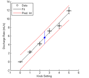
Figure 4. Prediction intervals of the pump calibration curve. The blue point represents the curve's predicted flow rate and uncertainty for a knob setting of 2.5.

The code to produce this figure is provided below.

 clear all
 close all
 knob = [0; 1; 2; 3; 4; 5];
 rate = [0.0; 2.3; 4.2; 7.2; 8.4; 11.9];
 err_knob = [0.2; 0.2; 0.2; 0.2; 0.2; 0.2];
 err_rate = [0.0; 0.3; 0.4; 0.5; 0.6; 0.7];
   
 figure; hold on;
 h1 = herrorbar(knob, rate, err_knob, 'ko');
 h2 = errorbar(knob, rate, err_rate, 'ko');
 axis square
 xlabel('Knob Setting');
 ylabel('Discharge Rate (mL/s)');
    
 fobj = fit(knob, rate, 'poly1');
 fknob = linspace(min(knob), max(knob), 50);
 frate = fobj(fknob);
 h3 = plot(fknob, frate, 'k-');
 fpi = predint(fobj, fknob);
 h4 = plot(fknob, fpi, 'r-');
 legend([h2 h3 h4(1)], {'Data', 'Fit', 'Pred. Int'}, 'Location', 'NorthWest');
    
 k_new = 2.5;
 r_new = fobj(k_new);
 pi_meas = predint(fobj, k_new);
 plot(k_new, r_new, 'bo', 'MarkerFaceColor', 'b');
 plot([k_new, k_new], pi_meas, 'b-');

Error of Fitted Curves

As we saw above, if we fit a set of experimental data to a theoretical form then we expect a certain amount of uncertainty on the fitted coefficients; we called this uncertainty the "95% confidence intervals on the coefficients." For the purposes of visualization (e.g., on a plot) these numbers aren't particularly helpful and instead we use a different kind of confidence interval called a "functional confidence interval," sometimes also called the "confidence interval of the fit" or the "fit confidence interval."

The equation to determine the fit confidence interval at any point on the regression curve is

\[y = \hat{y} \pm st_{\alpha, N-2} \left[\frac{1}{N} + \frac{n\left(x - \bar{x}\right)^2}{n \sum x_i^2 - \left(\sum x_i\right)^2}\right]^{1/2},\]

which is identical to the equation for the prediction interval except the "1" inside the square root has been omitted. As with the prediction interval, MATLAB gives us a built-in function to calculate this value so that we don't have to deal with this messiness. Even better, it's the same predint() function we already know and love but with a few extra settings, namely predint(fobj, xvals, level, intopt, simopt), where fobj is the fit object, xvals are the x-values at which to calculate the confidence interval, level is the desired confidence level (always 0.95 for this course), intopt is an interval option that tells MATLAB which interval--prediction of confidence--to compute, and simopt is an option that tells MATLAB to calculate the individual or simultaneous confidence intervals (we always use simultaneous).

For example, to calculate the fit confidence interval of calibration data (something you should not do, but it's convenient to do so here since we've already got all the data) we would use the following code:

ci_fit = predint(fobj, fknob, 0.95, 'functional', 'on');
h5 = plot(fknob, ci_fit, 'b-');    
legend([h2 h3 h4(1) h5(1)], {'Data', 'Fit', '95% Pred. Int.', '95% Conf. Int.'}, ...
   'Location', 'NorthWest');       
hold off

This code will produce the plot shown in Figure 5.

Figure 5. Confidence intervals (blue) for the pump calibration curve fit.

Note that the confidence interval is smaller than the prediction interval. This is because the confidence interval does not include the (predicted) random variation of a new variable; it is concerned only with the values already recorded. This is why I mentioned above that the fit confidence interval should not be included in calibration data, which are always concerned with the next data point. Fit confidence intervals, as described on the Plots and Tables page, should always be used when you perform a regression to compare experimental data to a theoretical form (e.g., rate laws in UV photocatalysis, characteristic curves in PEM fuel cells, mass transfer coefficients in reverse osmosis, and non-dimensional analyses in plate heat exchangers).

Interpolation

Interpolation is the tool we use when we have a table of data but the value we seek isn't explicitly listed in the table. For example, consider this abbreviated enthalpy table for steam (in kJ/kg) shown in Table 3.

P (bar)	T = 100 (°C)	T = 150 (°C)	T = 200 (°C)
0.5	2683	2780	2878
1.0	2676	2776	2875
5.0	419	632	2855

Suppose we need to know the enthalpy of steam at 1.0 bar and 163 °C: there's a row for 1.0 bar but no column for 163 °C, so what do we do? We interpolate!

Linear Interpolation

Linear interpolation is the most common form of interpolation and it assumes that the points given in a table are "connected" by straight lines. For example, consider the P = 1 bar row of Table 3 in graphical form:

fig1 here

The white circles are the data points given in Table 3, the red dashed line is a straight line between each point, and the red data point is the value at 163 °C that we wish to determine. Since the points are assumed to be connected by straight lines we can use similar triangles to determine the enthalpy value at 163 °C; graphically, the two triangles we need are shown in Figure 6.

fig2 here

The "similar triangles" principle applied to this situation is that the ratio of the arms of each triangle will be equivalent such that

\[\left(\frac{\textrm{rise}}{\textrm{run}} \right )_{\textrm{triangle 1}} = \left(\frac{\textrm{rise}}{\textrm{run}} \right )_{\textrm{triangle 2}}\]

Importantly, we know the x and y-values of all points in triangle 2 and all but one value for triangle 1, so we have one equation for one unknown:

\(\frac{2875-2776}{200-150}=\frac{H-2776}{163-150}\)

From this equation we calculate the unknown enthalpy as H = 2801.7 kJ/kg and this is what we call the interpolated value.

Another way to think of this process (and the one that I usually use) is to imagine a miniature table that contains only the points of interest:

T (°C)	H (kJ/kg)
150	2776
163	?
200	2875

Linear interpolation implies that (163-150)/(200-150) has to be equal to (?-2776)-(2875-2776), from which we can again determine the enthalpy as H = 2801.7 kJ/kg at 163 °C.

Double Interpolation

If the data pair you seek isn't listed on either the rows or columns of the table then you'll need to perform double interpolation. For example, suppose you've got the enthalpy table for steam (in kJ/kg) given in Table 3 but you need the enthalpy for P = 1.2 bar and T = 179 °C. The data given in the table cover this range but this particular temperature and pressure are not given. You could draw the similar triangles thing again but I think it's easier to show in in the tabular form as